jfunction – Guinness Stencil Problem

1 Problem Setup

The Modelling and Simulation Hub, Africa (MASHA) where I work has established a Data Science Masters programme with the Clinton Health Access Initiative (CHAI). The programme is designed to train data scientists to work on health data in Africa. Once a year the students and staff related to the programme will go to a pub or restaurant as a sort of informal initiation.

This year, while at the local pub, we noticed that the bartenders at the pub use stencils to sprinkle cocoa powder on the foam of the Guinness pints. The stencils are in various shapes and probably a few of us wondered what all of the shapes were. This intuitively reminded me of a video I had watched on Approximate Bayesian Computation (ABC) and I thought the question of how many stencils there are could be answered using this technique. Though incredibly lame, I felt inspired¹ to pose a question to the table:

Given the available data, how many stencils do we think the pub has?

Of course I should not have been surprised when someone quickly came back with “ask the pub”. I mean, this is absolutely the right answer but if we just asked the pub I wouldn’t have had the opportunity to demonstrate the use of ABC in this blog post.

2 Data Collection

As expected, we would like a nice sample in order to answer the question, at least enough to see some duplicate and some unique stencils. In total 4 draughts were ordered and 3 unique stencils were observed. This is all of the data we have but one of the strong points of ABC is it’s ability to work with “tiny data”.

Another thing we need to do is to define a prior distribution for the number of stencils. This is a bit tricky because the only prior knowledge we have on the number of stencils is that there are at least 3. I decided maybe a good prior to use is a triangular distribution with a minimum of 3, a maximum of 10 and a peak at 3. This is just a straight line from 3 being most probable to 10 being least probable. This is a bit arbitrary but that’s Bayes for you.

library(tidyverse)
dataRaw <- c(1, 2, 1, 3)
dataActual <- length(unique(dataRaw))

# Prior
sampleNumStencils <- function(a=3, b=10, c=3) {
  as.integer(triangle::rtriangle(1, a=a, b=b, c=c))
}

3 Model

The other thing we need to do is to define a generative model. This is a function that takes the true number of stencils in the pub and the number of draughts ordered then simulates the process of stencilling the draughts and finally returns the number of unique stencils observed.

# Generative model
getSample <- function(numStencils, numDraughts) {
  sampledStencils = sample(1:numStencils, numDraughts, replace = TRUE)
  numUniqueStencils = length(unique(sampledStencils))
  return(numUniqueStencils)
}

The last thing we need is a criteria for when a simulated dataset is “close enough” to the observed data. In our case we will accept nothing less than a perfect match².

# Criterion for when simulated data matches observed data
isMatch <- function(simulatedData, observedData) {
  return(simulatedData == observedData)
}

4 Approximate Bayesian Computation

We are now ready to run the ABC algorithm. We will run 100k simulations of some number of stencils in the pub and a random allocation of stencils to the 4 draughts. We accept the simulations that matched our observed data and use these to estimate the posterior distribution on the number of stencils in the pub.

numIterations <- 100000
matches <- integer(numIterations) # data management tip: pre-allocate memory for a vector
j <- 1
numDraughts <- length(dataRaw) # in our case there were 4 draughts ordered
dataActual <- length(unique(dataRaw))
for (i in 1:numIterations) {
  numStencils <- sampleNumStencils(a=dataActual, b=10, c=dataActual)
  simulatedData = getSample(numStencils, numDraughts)
  if (isMatch(simulatedData, dataActual)) {
    matches[[j]] <- numStencils
    j <- j+1
  }
}
matches <- matches[matches!=0] # data management: remove empty elements

We also want to get a point estimate of the number of stencils. We will use the median of the accepted simulations as our point estimate.

med = median(matches)

5 Results

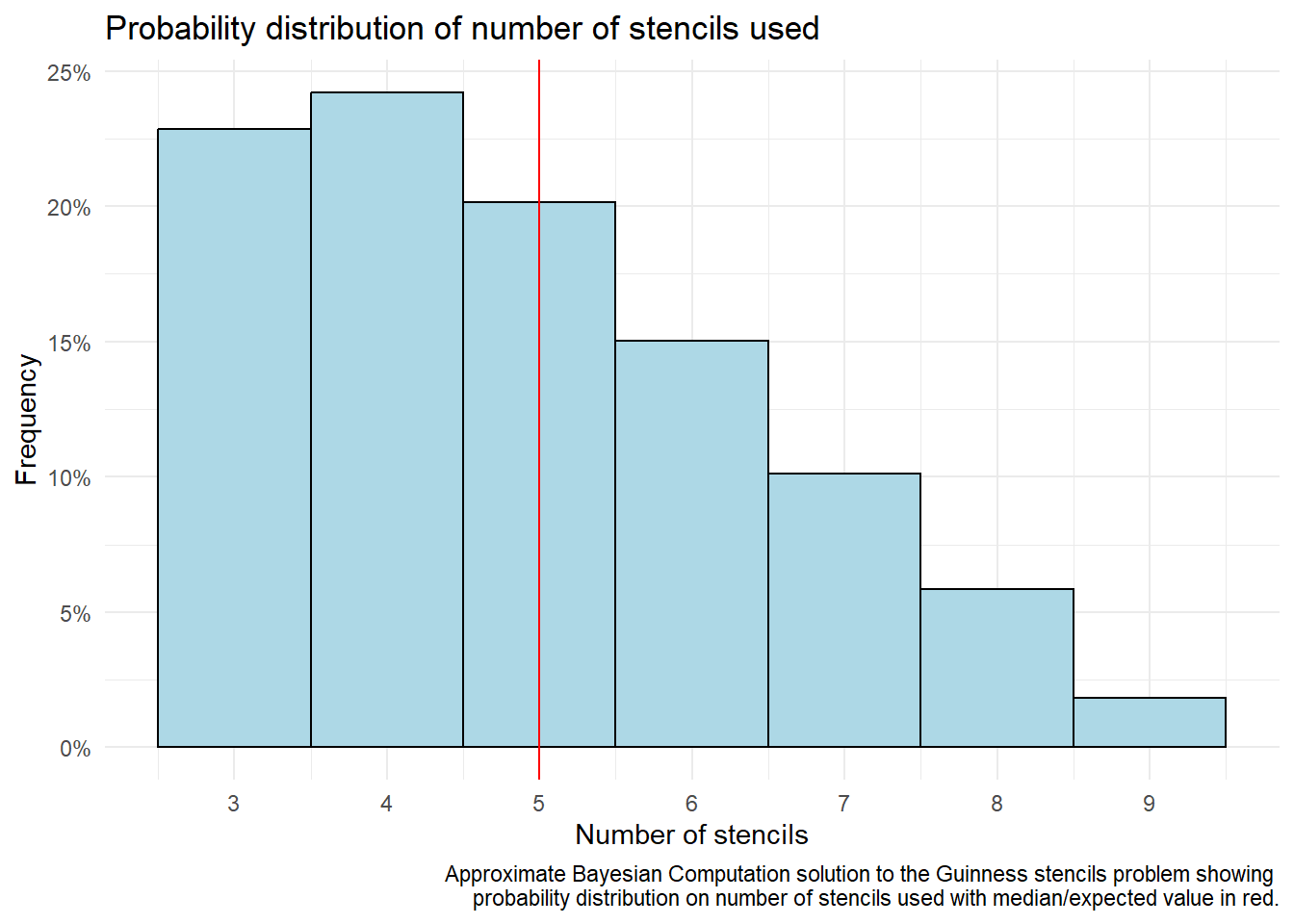
Lastly we can look at a plot of the resulting posterior distribution of the number of stencils together with our point estimate.

6 Conclusion

The ABC algorithm has estimated the number of stencils used at the pub to be 5. This is consistent with the observed data and the prior knowledge that there are at least 3 stencils and only a few draughts were ordered. We can do more though, we can say that we’re about 70% sure there are no more than 5 stencils in total. For more robust estimates though, we will need to go back to the pub.

I hope this blog post has given some insight into where ABC can be useful and how it works. It really isn’t complicated and the whole script for this problem came to 60 lines (including comments, white space and the setup code at the top). The video I linked is a great resource for learning more about ABC and I highly recommend it.

Footnotes

Perhaps this inspiration was partly due to something I learned a while back while sleuthing into the history of Statistics. The well known Students t-test is the invention of William Sealy Gosset who worked for the Guinness brewery in Dublin. He published under the pseudonym “Student” because Guinness did not want their competitors to know they were using statistics to improve their product.↩︎
Fun fact, we could have just done isMatch <- `==` but this is more readable and we might want to change the criteria in the future.↩︎