jfunction – Number 19

1 Rabbit Hole

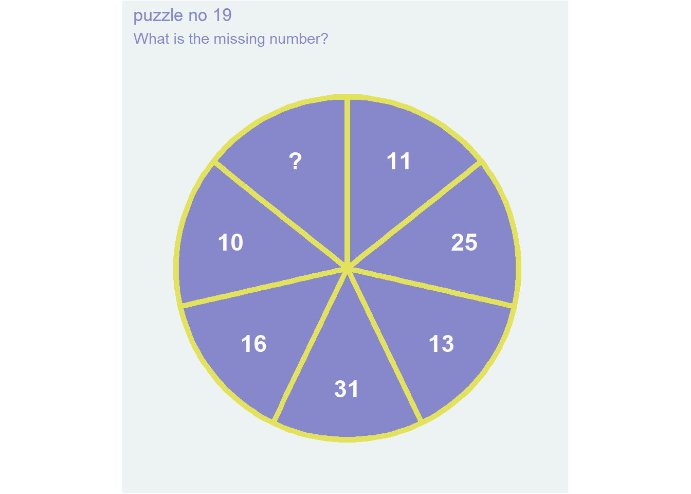
I found a deck of Mensa cards in the book shelf. Each card contains some logic-y puzzle. The first one I saw had “number 19” written at the top. I looked at it for a few seconds - a pie chart of sorts with numbers in each slice except for one containing a question mark. I brushed it off because of a certain mathematical trick which allows you to justify ANY answer to this question (I will describe it later). Putting my trick aside though, it still seemed confusing as to what the “right” answer might be. The approach did not come to me and I started wondering if the problem, which involves numbers, was even mathematical at all¹. I still wasn’t getting it though but I had an idea on how to explore the problem - more on all that in a minute.

When I looked through some of the others and I was satisfied that they were not so tough - generally there was some mathematical approach to solving them that I could see working out with some work so they didn’t really speak to me. This contrast begged me to reconsider my initial brushing off of that “number 19” I had seen first. The pull to reconsider the problem was enticing and I decided I can’t spare the time to bite… but maybe I could gnaw just a little?

2 Problem Statement

The problem was stated simply enough so I will reproduce it here:

nums = c(11,25,13,31,16,10,'?')
tbData = tibble(label=factor(nums,levels = nums)) %>%
  mutate(area=1)
ggplot(tbData, aes(x=label, y=area)) +
  geom_col(width=1, linewidth=2, color='#E2E25C',fill='#8787CB') +
  coord_polar("x", start=0, direction = 1) +
  geom_text(aes(label = label),
            position = position_stack(vjust=0.7),
            color='white',
            size=6,
            fontface = "bold") +
  labs(x = NULL, y = NULL,
       title="puzzle no 19",
       subtitle="What is the missing number?") +
  theme_classic() +
  theme(plot.background = element_rect(fill = "#EDF2F3"),
        panel.background = element_rect(fill = "#EDF2F3"),
        title = element_text(color='#8787CB'),
        axis.line = element_blank(),
        axis.text = element_blank(),
        axis.ticks = element_blank())

3 Mathematical Trick

As promised I will what my initial response to this sort of question is. Where you are asked to find “the missing number” you need to be able to justify why you put a given number as your answer. We often had this kind of question at school - fill in the missing number:

\(2,4,6,…\)

In this case you are invited to put \(8\) down and say that the pattern is just adding \(2\) each time. That has to be the right answer, right? Well, yes and no. Your framework at that point is arithmetic and geometric sequences so there are only two possible approaches you’re meant to consider: either a common difference or a common ratio should be seen between numbers.

In an arithmetric sequence we have \(T_{n+1} = T_{n}+d\) for some \(d\). The solution for the n’th term is just \(T_n = T_0 + n d\) . This can be read as “The nth term is the zeroith term plus \(n\) copies of \(d\)”.

In a geometric sequence we have \(T_{n+1} = r T_{n}\) for some \(r\). The solution for the n’th term is just \(T_n = r^n T_0\) . This can be read as “The nth term is the zeroith term multiplied \(n\) times by \(r\)”.

In fact there is a nice generalisation of these called the arithmetico-geometric sequence where \(T_n = r^n(a+nd)\). If you look these up online you will see the convention is to start at 1 not 0² so \(n-1\) is used instead of \(n\).

Alas, we have digressed, I wanted to show another valid answer to the \(2,4,6,...\) question. Suppose you want to put \(10\) there instead. How can you justify that? One way is with polynomials.

3.1 Fitting with polynomials

Consider 2 points \((0,2)\) and \((1,4)\). You can fit a line through two points and in this case its \(y=2x+2\). I need to labour a point here, we could have solved this by noting our 2 constraints:

\[ \begin{matrix} y(0) = y_0 = m x_0+c \\ y(1) = y_1 = m x_1+c \end{matrix} \]

We could even write this in matrix form:

\[ \begin{pmatrix} y_0\\ y_1 \end{pmatrix} = \begin{pmatrix} 1 & x_0\\ 1 & x_1 \end{pmatrix} \begin{pmatrix} c\\ m \end{pmatrix} \]

We know the x and y values and need to solve for the coefficients \(c\) and \(m\). This is easily done by left multiplying both sides by the inverted matrix which can be calculated using many methods supposing it is invertible³. The point is that we can fit a line through two points and we can justify any third number we put down by saying it is the value of the line at that point.

What if we have 3 points? Well, you can fit something with an \(x^2\) term in there:

\[ \begin{pmatrix} y_0\\ y_1\\ y_2 \end{pmatrix} = \begin{pmatrix} 1 & x_0 & x_0^2\\ 1 & x_1 & x_1^2\\ 1 & x_2 & x_2^2 \end{pmatrix} \begin{pmatrix} c\\ b\\ a \end{pmatrix} \]

It’s getting a bit awkward to name the coefficients but you get the point right? There is a way of fitting a polynomial of degree 2 through any three points you specify. If we have the \(x\) values of these points line up with the indices in our sequences above you can justify putting any 3rd number down by using a polynomial of degree 2. In general then, by inverting Vandermonde matrices (as these are called) you can answer the question with any number you like. For a 3x3 we can get the explicit inverse:

\[ \begin{pmatrix} \frac{x_1x_2}{(x_0-x_1)(x_0-x_2)} & \frac{x_0x_2}{(x_1-x_0)(x_1-x_2)} & \frac{x_0x_1}{(x_2-x_0)(x_2-x_1)}\\ -\frac{x_1+x_2}{(x_0-x_1)(x_0-x_2)} & -\frac{x_0+x_2}{(x_1-x_0)(x_1-x_2)} & -\frac{x_0+x_1}{(x_2-x_0)(x_2-x_1)}\\ \frac{1}{(x_0-x_1)(x_0-x_2)} & \frac{1}{(x_1-x_0)(x_1-x_2)} & \frac{1}{(x_2-x_0)(x_2-x_1)} \end{pmatrix} \]

In the above we generally have \(x_i=i+1\) so that \(x_0=1, x_1=2, x_2=3\). That means we get to simplify this a whole lot and solve for the coefficients directly as:

\[ \begin{pmatrix} c\\ b\\ a \end{pmatrix} = \frac{1}{2}\begin{pmatrix} 6 & -6 & 2\\ -5 & 8 & -3\\ 1 & -2 & 1 \end{pmatrix} \begin{pmatrix} y_0\\ y_1\\ y_2 \end{pmatrix} \]

If you follow this for example when \(y_0=2\), \(y_1=4\) you will find an interesting construction: \(T_n = \frac{y_2-6}{2}(n^2-3n+2) + 2n\)

Interestingly the \(n^2-3n+2\) polynomial evaluates to 0 for the first two points so the expression is effectively just \(2n\) there. In the case of the third point the \(2n\) is like an error and the \(y_2-6\) “corrects” for it. Not sure I’m explaining myself well right now but the point I’m driving at is that I suspect this idea can be generalised so one can create a “yummy” part and a “yucky” part for these sorts of problems and I wanted to make a note of it.

3.2 Extension: Saying NO

You can even solve it as \(2,4,6,NO\). This is because \(NO\) is a valid number expressed in base 25. In this case its decimal form is 599 which we can verify with some code⁴:

num = "NO"
# Convert the input string to uppercase to handle lowercase input
num <- toupper(num)

# Define a vector of characters representing the base 25 digits
digits <- c(1:9,LETTERS)[1:(25-1)]

# Initialize a variable to store the decimal value
decimal <- 0

# Loop through each character in the input string
for (i in seq(nchar(num))) {
  # Get the current character
  char <- substr(num, i, i)
  
  # Get the corresponding base 25 digit value
  value <- match(char, digits)

  # Add the digit value times 25^exponent to the decimal value
  exponent <- nchar(num) - i
  decimal <- decimal + value * 25^exponent
}
decimal

[1] 599

For questions giving 3 numbers and asking for a fourth we’d find the inverse Vandermonde as:

\[ \frac{1}{6} \begin{pmatrix} 24 & -36 & 24 & -6\\ -26 & 57 & -42 & 11\\ 9 &-24 & 21 &-6\\ -1 & 3 & -3 & 1 \end{pmatrix} \tag{1}\]

We can then multiply this by the asserted \(Tn\) values to solve for the (better named) coefficients of our 4th order polynomial and solve in terms of \(NO\) to get:

\[ \begin{pmatrix} \alpha_0\\ \alpha_1\\ \alpha_2\\ \alpha_3 \end{pmatrix} = \frac{1}{6} \begin{pmatrix} 24 & -36 & 24 & -6\\ -26 & 57 & -42 & 11\\ 9 &-24 & 21 &-6\\ -1 & 3 & -3 & 1 \end{pmatrix} \begin{pmatrix} 2\\ 4\\ 6\\ NO \end{pmatrix} = \frac{1}{6} \begin{pmatrix} -6(NO-8)\\ 11(NO-8)+12\\ -6(NO-8)\\ (NO-8) \end{pmatrix} = \begin{pmatrix} -\gamma\\ \frac{11}{6}\gamma+2\\ -\gamma\\ \frac{1}{6}\gamma \end{pmatrix} \]

where I’ve obviously just introduced \(\gamma=591\) for simplicity. Then:

\[ T_n = \alpha_3n^3 +\alpha_2n^2 +\alpha_1n^1 +\alpha_0 =\gamma\left(\frac{1}{6}n^3 - n^2 + (\frac{11\gamma+12}{6\gamma})n - 1\right) \tag{2}\]

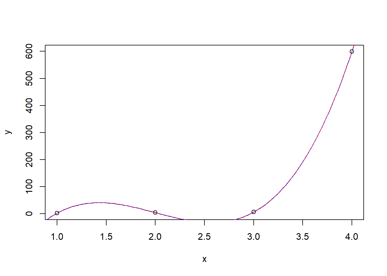
A sweet hack to find the coefficients of your polynomial is just to do a linear model. Here’s code comparing our analytic solution to one derived using the lm function:

# Some helper functions:
coefTn = function(NO=599) {
  # Get the coefficients directly from our equations
  gam=NO-8
  list(a0 = -gam,
       a1 = ((11*gam+12)/(6)),
       a2 = -gam,
       a3 = gam/6)
}
coefLm = function(fit){
  # Get the coefficients from a linear model with same formatting as coefTn function
  result = as.list(unname(coef(fit)))
  names(result) = paste0('a',seq(from=0,to=3,by=1))
  result
}
Tn = function(n, NO=599) {
  # Call Tn using the coefficients we got from our inverted Vandermonde
  with(coefTn(NO=NO), {
    a3*n^3 + a2*n^2 + a1*n + a0
  })
}

# Plot the points:
NO = 599
y = c(2,4,6,NO)
x = seq_along(y)
plot(x, y, xlim=range(x), ylim=range(y))

# Plot the analytically derived polynomial as well as the one derived from lm:
xx <- seq(min(x)-1, max(x)+2, length.out=250)
fit = lm(y ~ 1 + I(x) + I(x^2) + I(x^3))
yy.lm = predict(fit, data.frame(x=xx))
yy.Tn = Tn(xx, NO=NO)

lines(xx, yy.lm, col='blue')
lines(xx, yy.Tn, col='red', lt=2)

Let’s check the coefficients we derived for Tn match with the linear models coefficients:

tibble(
  coef=names(coefLm(fit)),
  coef_lm = coefLm(fit),
  coef_Tn = coefTn(NO=NO)
) %>%
  unnest(contains('_'))

# A tibble: 4 × 3
  coef  coef_lm coef_Tn
  <chr>   <dbl>   <dbl>
1 a0     -591.   -591  
2 a1     1086.   1086. 
3 a2     -591.   -591  
4 a3       98.5    98.5

Another quick note, in this case we’ve done a trick using polynomials which are a series incorporating the \(x^n\) basis functions. We could have used for example the \(\sin(nx)\) basis functions in which case we’d find ourselves looking into Fourier analysis. I just wanted to mention that.

Lastly, Bernoulli numbers are another topic intersecting with Vandermonde matrices in an interesting way, but that’s quite tangential at this point so I will leave it at that for now.

Anyway, this has been a long tangent just to say you can technically put any number there. So when I saw the problem initially I sort of brushed it off with this trick. This is disingenuous though - usually when you solve a problem you get a kind of feeling like “oh yeah, this must be the answer” not “technically any answer is valid even the word \(NO\)”. That’s just arm-folding know-it-all tomfoolery and I won’t have it. I simply must gnaw.

4 Gnawwing: Drawing lines

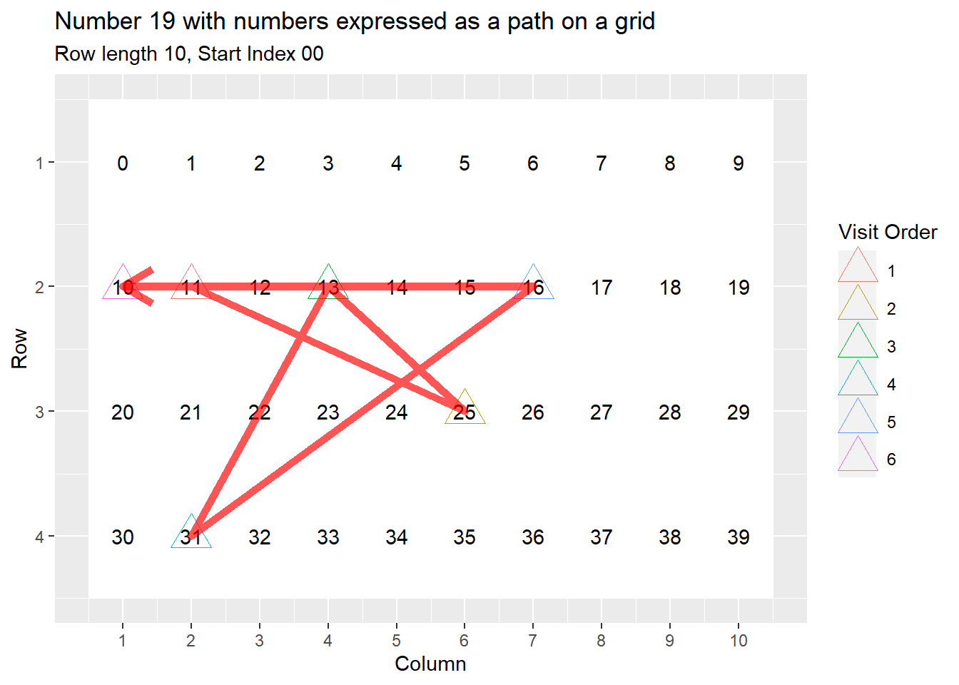
So gnawwing at “number 19” proved useful and satisfying - for my first attempt I thought to simply trace the displayed numbers in order on a grid.

The result wasn’t particularly interesting but I wondered if perhaps a pattern wasn’t emerging because I had imposed some hidden constraint. For example being in base 10 is potentially too restrictive. I therefore allowed the grid size to vary as well as the offset.

makeTbGrid <- function(startWith=0, rowLength=10) {
  validNums = as.integer(nums[nums!='?'])
  minimumNumbersRequired = max(validNums-startWith+1)
  rowsRequired = as.integer(ceiling(minimumNumbersRequired/rowLength))
  cellsRequired = rowLength*rowsRequired
  endWith = startWith+cellsRequired-1
  tbAllNums = expand.grid(col=1:rowLength, row=1:rowsRequired) %>%
    as_tibble() %>%
    rowid_to_column() %>%
    mutate(i=startWith+rowid-1) %>%
    select(i,row,col)
}

makeTbNums <- function(startWith=0, rowLength=10) {
  validNums = as.integer(nums[nums!='?'])
  tbGrid = makeTbGrid(startWith, rowLength)
  tbNums = tibble(i=validNums) %>%
    left_join(tbGrid, by = join_by(i))
  tbNums
}

makePlot <- function(startWith, rowLength) {
  tbGrid <- makeTbGrid(startWith = startWith, rowLength = rowLength)
  tbNums <- makeTbNums(startWith = startWith, rowLength = rowLength) %>%
    rowid_to_column()
  
  ggplot(tbGrid)+
    aes(x=col,y=row)+
    geom_tile(fill='white')+
    geom_text(aes(label=i))+
    geom_point(data=tbNums,
               mapping=aes(x=col,y=row,color=as_factor(as.character(rowid))),
               size=7,
               shape=2)+
    geom_path(data=tbNums,
              mapping=aes(x=col,y=row),
              color='#FF0000AA',
              linewidth=2,
              arrow = arrow(ends='last'))+
    scale_color_discrete()+
    scale_x_continuous(breaks=1:max(tbGrid$col))+
    scale_y_continuous(breaks=1:max(tbGrid$row))+
    scale_y_reverse()+
    labs(x='Column',y='Row',color='Visit Order',
         title="Number 19 with numbers expressed as a path on a grid",
         subtitle=glue::glue("Row length {sprintf(rowLength, fmt='%02d')}, Start Index {sprintf(startWith, fmt='%02d')}"))
}

# I made a lot of plots and looked through them...
# for (rowLength in seq(2,20)) {
#   for (startWith in seq(0,rowLength-1)) {
#     filename = glue::glue("number19_rl{sprintf(rowLength, fmt='%02d')}_sw{sprintf(startWith, fmt='%02d')}.png")
#     print(filename)
#     plt = makePlot(startWith=startWith, rowLength=rowLength)
#     ggsave(plot = plt, filename=filename)
#   }
# }
makePlot(startWith = 0, rowLength = 10)  # the most natural looking grid

Scale for y is already present.
Adding another scale for y, which will replace the existing scale.

After playing with these plots for a bit an obvious pattern jumped out at me. When I went to try confirm that the number that jumped out fits, another pattern showed itself on the question card. I will just leave it at that so you can play around and discover what I mean yourself. This process of generating some hypothesis and when you investigate it something else comes out right too is discussed by Richard Feynman in his book “Surely you’re Joking, Mr. Feynman!”. That was an interesting book.

When you’re ready to come back to the question see Section 2.

Footnotes

Sometimes these problems use numbers to lure you into mathematical thinking but then you realise the approach is something like saying the numbers out loud and interpreting what you’re saying in some way, eg Look-and-say sequence - Wikipedia ↩︎
An interesting discussion on whether to index from 0 or by 1 is found here.↩︎
The matrix is invertible if the determinant is non-zero and one method used to invert matrices is Gaussian elimination. Three points could be in a line meaning there’s no strictly order 2 polynomial that fits them and the coefficient on the x^2 term is zero - this would make the determinant zero.↩︎
I wanted this to be easier - I wondered why base R doesn’t come with integer base conversion built in. eg in python this is as simple as int('NO',25)↩︎